Analysis of diff cost Marginal cost,Standard Cost?
Marginal cost is the change in the total cost when the quantity
produced is incremented by one. That is, it is the cost of producing one
more unit of a good. For example, let us suppose:
Variable cost per unit     = Rs 25
Fixed cost                 = Rs 1,00,000
Cost of 10,000 units       = 25 × 10,000 = Rs 2,50,000
Total Cost of 10,000 units = Fixed Cost + Variable Cost
                           = 1,00,000 + 2,50,000
                           = Rs 3,50,000
Total cost of 10,001 units = 1,00,000 + 2,50,025
                           = Rs 3,50,025
Marginal Cost              = 3,50,025 – 3,50,000
                           = Rs 25
Need for Marginal Costing
Let us see why marginal costing is required:- Variable cost per unit remains constant; any increase or decrease in production changes the total cost of output.
- Total fixed cost remains unchanged up to a certain level of production and does not vary with increase or decrease in production. It means the fixed cost remains constant in terms of total cost.
- Fixed expenses exclude from the total cost in marginal costing technique and provide us the same cost per unit up to a certain level of production.
Features of Marginal Costing
Features of marginal costing are as follows:- Marginal costing is used to know the impact of variable cost on the volume of production or output.
- Break-even analysis is an integral and important part of marginal costing.
- Contribution of each product or department is a foundation to know the profitability of the product or department.
- Addition of variable cost and profit to contribution is equal to selling price.
- Marginal costing is the base of valuation of stock of finished product and work in progress.
- Fixed cost is recovered from contribution and variable cost is charged to production.
- Costs are classified on the basis of fixed and variable costs only. Semi-fixed prices are also converted either as fixed cost or as variable cost.
Ascertainment of Profit under Marginal Cost
‘Contribution’ is a fund that is equal to the selling price of a product less marginal cost. Contribution may be described as follows:Contribution = Selling Price – Marginal Cost Contribution = Fixed Expenses + Profit Contribution – Fixed Expenses = Profit
Income Statement under Marginal Costing
|
Income Statement
For the year ended 31-03-2014
|
||
| Particulars | Amount | Total |
| Sales | 25,00,000 | |
| Less: Variable Cost: | ||
| Cost of goods manufactured | 12,00,000 | |
| Variable Selling Expenses | 3,00,000 | |
| Variable Administration Expenses | 50,000 | |
| 15,50,000 | ||
| Contribution | 9,50,000 | |
| Less: Fixed Cost: | ||
| Fixed Administration Expenses | 70,000 | |
| Fixed Selling Expenses | 1,30,000 | 2,00,000 |
| 7,50,000 | ||
Advantages of Marginal Costing
The advantages of marginal costing are as follows:- Easy to operate and simple to understand.
- Marginal costing is useful in profit planning; it is helpful to determine profitability at different level of production and sale.
- It is useful in decision making about fixation of selling price, export decision and make or buy decision.
- Break even analysis and P/V ratio are useful techniques of marginal costing.
- Evaluation of different departments is possible through marginal costing.
- By avoiding arbitrary allocation of fixed cost, it provides control over variable cost.
- Fixed overhead recovery rate is easy.
- Under marginal costing, valuation of inventory done at marginal cost. Therefore, it is not possible to carry forward illogical fixed overheads from one accounting period to the next period.
- Since fixed cost is not controllable in short period, it helps to concentrate in control over variable cost.
Planned cost is a key for effective cost control which is not provided by historical cost concepts. The standard costing system was developed to overcome the drawbacks of the historical costing system. Since historical costing deals only with the actual costs incurred, it is not an effective device of cost control.
Standard costing tells us what should be the cost of the product and if the actual cost exceeds the projected cost, the standard costing system can point to the reason of deviation.
Points Related to Standard Costing
- Standard costing includes pre-determination of costs under specific working conditions.
- In this process, the standard quantity of machine time, labor time, and material is calculated and the future market trend for price standards is analyzed.
- Standard costing helps in variance analysis.
- Along with fixation of sale price, it also provides valuation of stock and work in progress.
- Material, labor, and overheads cost are ascertained.
- Actual cost is measured.
Standard Cost Card
Format
| Standard Cost Card
No ... ... ... ... Product... ... ... ... Date of setting Standard... ... ... ... |
|||
| Element of Cost | Quantity of Hours | Rate Rs. | Standard Cost |
|
1. Direct Material
Material A
Material B
|
400 units
100 units |
5.00
4.00
|
2,000
400
|
| 500 units | 2,400 | ||
| Less: Normal Loss 5% | 25 units | Scrap Value | 400 |
| Normal Output | 475 units | 2,000 | |
| 2. Direct Labour | 100 hrs | 20 | 200 |
| 3. Overheads | |||
When the actual cost differs from the standard cost, it is called variance. If the actual cost is less than the standard cost or the actual profit is higher than the standard profit, it is called favorable variance. On the contrary, if the actual cost is higher than the standard cost or profit is low, then it is called adverse variance.
Each element of cost and sales requires variance analysis. Variance is classified as follows:
- Direct Material Variance
- Direct Labor Variance
- Overhead Variance
- Sales Variance
Direct Material Variance
Material variances can be of the following categories:- Material Cost Variance
- Material Price Variance
- Material Usage Variance
- Material Mix Variance
- Material Yield Variance
| Material Cost Variance | |
|
Standard cost of materials for actual output – Actual cost of material used
Or
Material price variance + Material usage or quantity variance
Or
Material price variance + Material mix variance + Material yield variance
|
|
| Material Price Variance | |
|
Actual usage ( Standard Quantity Price – Actual Unit Price) Actual Usage = Actual Quantity of material (in units) used Standard Unit Price = Standard Price of material per unit Actual Unit Price = Actual price of material per unit |
|
| Material Usage or Quantity Variance | |
|
Material usage or Quantity variance :
Standard price per unit (Standard Quantity – Actual Quantity ) |
|
| Material Mix Variance | |
|
Material mix variance arises due to the difference between the
standard mixture of material and the actual mixture of Material mix. Material Mix variance is calculated as a difference between the standard prices of standard mix and the standard price of actual mix. If there is no difference between the standard and the actual weight of mix, then:
Standard unit cost (Standard Quantity – Actual Quantity )
Or
Standard Cost of Standard Mix – Standard cost of Actual Mix
Sometimes due to shortage of a particular type of material, standard is revised; then:
Standard unit cost (Revised Standard Quantity – Actual Quantity)
Or
Standard cost of revised Standard Mix – Standard Cost of Actual mix
If the actual weight of mix differs from the standard weight of mix, then:
Standard cost of revised standard mix ×
Total weight of actual mix
mixTotal weight of revised standard mix
|
|
| Material Yield Variance | |
|
When the standard and the actual mix do not differ, then Yield Variance = Standard Rate × (Actual Yield – Standard Yield)
Standard Rate =
Standard cost of standard mix
Net standard output (i.e.Gross output−Standard loss)
|
Direct Labor Variance
Direct labor variances are categorized as follows:- Labor Cost Variance
- Labor Rate of Pay Variance
- Total Labor Efficiency Variance
- Labor Efficiency Variance
- Labor Idle Time Variance
- Labor Mix Variance or Gang Composition Variance
- Labor Yield Variance or Labor Efficiency Sub Variance
- Substitution Variance
| Labor Cost Variance | ||||||||||||||||||||||||||||||||||||||||||
|
Standard Cost of Labor – Actual Cost of Labor
|
||||||||||||||||||||||||||||||||||||||||||
| Labor Rate of pay Variance | ||||||||||||||||||||||||||||||||||||||||||
|
Actual Time taken × (Standard Rate – Actual Rate)
|
||||||||||||||||||||||||||||||||||||||||||
| Total Labor Efficiency Variance | ||||||||||||||||||||||||||||||||||||||||||
|
Standard rate × (Standard time – Actual time)
|
||||||||||||||||||||||||||||||||||||||||||
| Labor Efficiency Variance | ||||||||||||||||||||||||||||||||||||||||||
|
Standard Rate (Standard time for actual output – Actual time worked)
|
||||||||||||||||||||||||||||||||||||||||||
| Labor Idle Time Variance | ||||||||||||||||||||||||||||||||||||||||||
|
Idle Time Variance = Abnormal Idle Time × Standard Rate Total Labor Cost Variance = Labor rate of Pay variance + Total labor Efficiency Variance Total Labor Efficiency Variance = Labor Efficiency Variance + Labor Idle Time Variance |
||||||||||||||||||||||||||||||||||||||||||
| Labor Mix Variance or Gang Composition Variance | ||||||||||||||||||||||||||||||||||||||||||
|
If actual composition of labor is equal to standard: LMV = Standard Cost of Standard Composition (for Actual time taken) – Standard Cost of Actual Composition (for Actual time worked) If standard composition of labor revised due to shortage of any specific type of labor but the total actual time is equal to the total standard time: LMV = Standard Cost of Revised Standard Composition (for Actual Time Taken) – Standard Cost of Actual Composition (for Actual Time Worked) If actual and standard time of labor differs:
=
In case the Standard is revised and there is a difference in the total Actual and the Standard time:
Total time of actual labor composition
Total time of standard labor composition
× Std.cost of std.composition − Std.cost of actual composition
=
Total time of actual labor composition
Total time of revised std.labor composition
× Std.cost of (revised std.composition − actual composition)
|
||||||||||||||||||||||||||||||||||||||||||
| Labor Yield Variance | ||||||||||||||||||||||||||||||||||||||||||
| Std. Labor Cost per unit × (Actual Yield In units – Std. Yield in units expected from Actual time worked on production) | ||||||||||||||||||||||||||||||||||||||||||
| Substitution Variance | ||||||||||||||||||||||||||||||||||||||||||
| (Actual hrs × Std. Rate of Std. Worker) – (Actual hrs × Std.Rate actual worker)Cost-Volume-Profit (CVP) Analysis is also known as Break–Even
Analysis. Every business organization works to maximize its profits.
With the help of CVP analysis, the management studies the co-relation of
profit and the level of production. CVP analysis is concerned with the level of activity where total sales equals the total cost and it is called as the break-even point. In other words, we study the sales value, cost and profit at different levels of production. CVP analysis highlights the relationship between the cost, the sales value, and the profit. AssumptionsLet us go through the assumptions for CVP analysis:
Marginal Cost EquationEquations for elements of cost are as follows:Sales = Variable costs + Fixed Expenses ± Profit /Loss
Or
Sales – Variable Cost = Fixed Expenses ± Profit /Loss
Or
Sales – Variable Cost = Contribution
It is necessary to understand the following four concepts, their
calculations, and applications to know the mathematical relation between
cost, volume, and profit:
ContributionContribution = Sales – Marginal CostWe have already discussed contribution in Marginal Costing topic above. Profit-Volume RatioProfit / Volume (P/V) ratio is calculated while studying the profitability of operations of a business and to establish a relation between Sales and Contribution. It is one of the most important ratios, calculated as under:
P⁄V Ratio =
Contribution
Sales
=
Fixed Expenses+Profit
Sales
=
Sales−Variable Cost
Sales
=
The P/V Ratio shares a direct relation with profits. Higher the P/V ratio, more the profit and vice-a-versa.
Change in profits of Contributions
Change in Sales
Break-Even PointWhen the total cost of executing business equals to the total sales, it is called break-even point. Contribution equals to the fixed cost at this point. Here is a formula to calculate break-even point:
B.E.P (in units) =
Total Fixed Expenses
Selling Price per Unit − Marginal Cost per Unit
=
Break-even point based on total sales:
Total Fixed Expenses
Contribution per Unit
=
Calculation of output or sales value at which a desired profit is earned:
Fixed Cost
P⁄V Ratio
=
Fixed Expenses + Desired Profit
Selling Price per Unit − Marginal Cost per Unit
=
Fixed Expenses + Desired Profit
Contribution per Unit
Composite Break Even PointA company may have different production units, where they may produce the same product. In this case, the combined fixed cost of each productions unit and the combined total sales are taken into consideration to find out BEP.
Margin of SafetyExcess of sale at BEP is known as margin of safety. Therefore,Margin of safety = Actual Sales − Sales at BEPMargin of safety may be calculated with the help of the following formula:
Margin of Safety =
Profit
P⁄V Ratio
=
Profit
Contribution per Unit
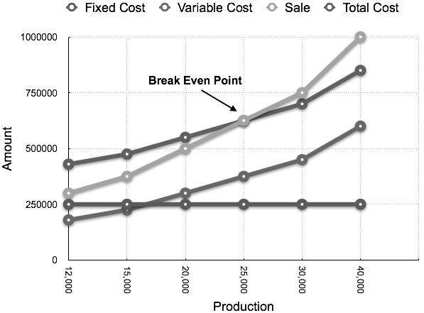
Break-Even ChartBreak-Even Chart is the most useful graphical representation of marginal costing. It converts accounting data to a useful readable report. Estimated profits, losses, and costs can be determined at different levels of production. Let us take an example.ExampleCalculate break-even point and draw the break-even chart from the following data:Fixed Cost = Rs 2,50,000 Variable Cost = Rs 15 per unit Selling Price = Rs 25 per unit Production level in units 12,000, 15,000, 20,000, 25,000, 30,000, and 40,000.Solution:
B.E.P =
Fixed Cost
Contribution per unit
=
Rs 2,50,000
Rs 10 × (Rs 25 - Rs 15)
= 25,000 units
At production level of 25,000 units, the total cost will be Rs 6,25,000.(Calculated as (25000 × 14) + 2,50000)
 | ||||||||||||||||||||||||||||||||||||||||||
Comments
Post a Comment